Generalised $f$-Mean Aggregation for Graph Neural Networks

Introduction

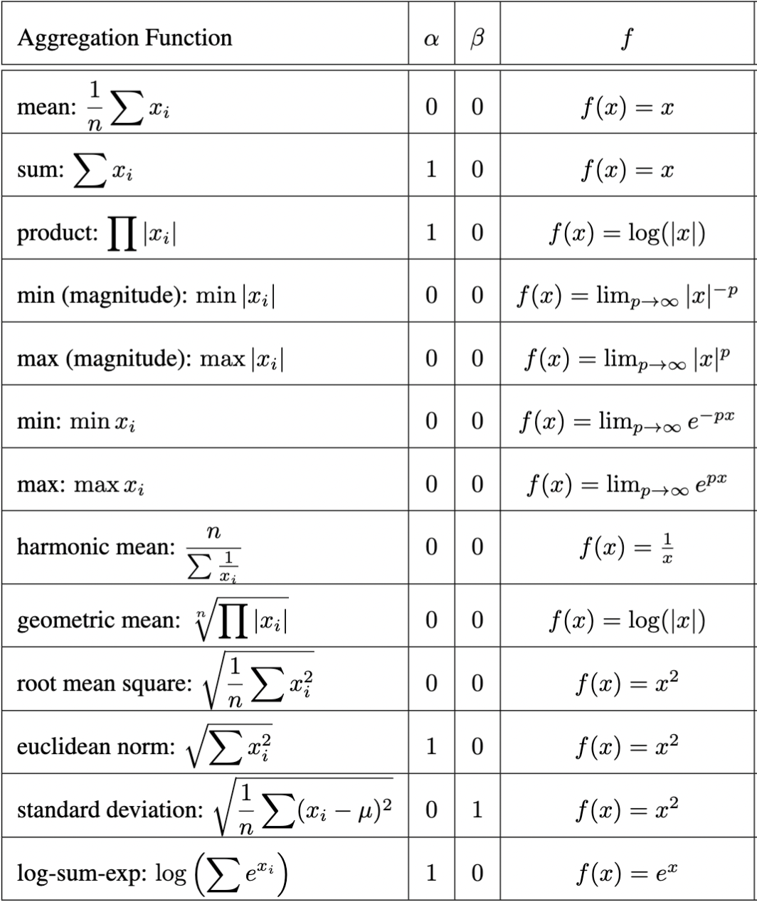
GenAgg is an aggregator that parametrises the function space of all standard aggregators. It is learnable, allowing it to converge to the most appropriate aggregator for a given problem. It is given by the following formula: $$\bigoplus_{x_i \in \mathcal{X}} x_i = f^{-1} \left( n^{\alpha-1} \sum_{x_i \in \mathcal{X}} f(x_i - \beta \mu) \right)$$ where $x_i$ are the inputs, $n=|\mathcal{X}|$ is the cardinality of the input, and $\mu=\mathrm{mean}(\mathcal{X})$. It is parametrised by a learnable invertible function $f$, and scalars $\alpha$ and $\beta$. The parametrisation of an aggregation function under GenAgg can be used for explainability, as each parameter carries a unique purpose:

• $f$: While aggregators might appear difficult to analyse, GenAgg shows that they can be represented by a unique scalar-valued function $f$. Interestingly, the most fundamental aggregation functions (sum, product, log-sum-exp, etc) tend to map to the most fundamental scalar-valued mathematical functions ( $x^p$, $e^x$, $\log(x)$ ). The aggregator corresponding to any function $f$ can be analysed by considering the sign and magnitude of $f(x_i)$. The sign denotes if a given $x_i$ increases ($f(x)>0$) or decreases ($f(x_i) < 0$) the output. On the other hand, the magnitude $|f(x_i)|$ can be interpreted as the relative impact of that point on the output. For example, the parametrisation of product is $f(x)=\log(|x|)$, which implies that a value of $1$ has no impact on the output since $|\log(|1|)|=0$, and extremely small values $\epsilon$ have a large impact, because $\lim_{\epsilon \to 0} |\log(|\epsilon|)| = \infty$. Indeed, $1$ is the identity element under multiplication, and multiplying by a small value $\epsilon$ can change the output by many orders of magnitude.
• $\alpha$: This is a scaling factor for GenAgg. It determines if the output is dependent on the number of inputs. For example, given $f(x) = x$, $\alpha=0$ denotes a mean, and $\alpha=1$ denotes a sum. Similarly, if $f(x) = \log|x|$, then $\alpha=0$ denotes a product and $\alpha=1$ denotes the geometric mean (i.e., the n-th root of the product).
• $\beta$: The $\beta$ parameter enables GenAgg to calculate centralised moments, which are quantitative measures of the distribution of the input $\mathcal{X}$. The first raw moment of $\mathcal{X}$ is the mean $\mu = \frac{1}{n}\sum{x_i}$, and the $k$-th central moment is given by $\mu_k = \sum{(x_i-\mu)^k}$. With the addition of $\beta$, it becomes possible for GenAgg to represent $\sqrt[k]{\mu_k}$, the $k$-th root of the $k$-th central moment. For example, for $k=2$, this quantity is the standard deviation. In general, the $\beta$ parameter can be understood as an indicator for whether an aggregator operates over the inputs themselves ($\beta=0$), or the variation between the inputs ($\beta=1$).

Installation

cd generalised-aggregation
pip install -e .

Basic Usage

GenAgg extends the torch_geometric definition of an Aggregation function. It uses the same sparse format as torch_scatter, allowing batched computation of aggregations with variable input sizes. Each element y[j] of the output will yield the aggregation of all input elements x[i] such that index[i]=j. In this example, we use the parametrisation f(x) = x with a = 0 and b = 0, which results in a mean aggregation.

import torch
from genagg import GenAgg
in_size = 8 # number of input nodes
out_size = 4 # number of output nodes
dim = 2 # dimension of each node
x = torch.randn(in_size, dim) # input
index = torch.randint(low=0, high=out_size, size=(in_size,)) # the output node for each input node to aggregate into
class Identity:
    def forward(self, x):
        return x
    def inverse(self, x):
        return x
agg = GenAgg(f=Identity(), a=torch.tensor(0.), a=torch.tensor(0.)) # initialise the aggregator
y = agg(x=x, index=index) # compute the output
print("x:", x)
print("index:", index)
print("y:", y.detach())

x: tensor([[-1.8775, -0.1037],
          [-0.2848,  0.3936],
          [-2.0698, -0.5925],
          [ 0.3421,  0.4746],
          [-1.4214,  0.1878],
          [ 0.6762,  0.1140],
          [-1.2734, -1.8754],
          [-0.2148,  1.8237]])

index: tensor([1, 0, 0, 0, 1, 0, 3, 3])

y: tensor([[-0.3341,  0.0974],
          [-1.6495,  0.0420],
          [ 0.0000,  0.0000],
          [-0.7441, -0.0259]])

GenAgg can also be used with dense inputs, in the same way one would compute torch.sum. In this example, we leave the f parameter blank, allowing it to be learned with an autoencoder-based invertible network MLPAutoencoder. However, note that the forward and inverse networks start off randomly initialised. The a and b parameters are initialised to zero and set to be learnable by default (however, if they are given a value like in the example above, they are set to be non-learnable).

x = torch.rand(4,2)
agg = GenAgg()
y = agg(x, dim=-1)
print("x:", x)
print("y:", y.detach())

x: tensor([[0.0908, 0.3474],
          [0.4259, 0.2529],
          [0.4894, 0.3151],
          [0.7059, 0.9566]])

y: tensor([[-0.2494],
          [ 0.7020],
          [ 0.8240],
          [ 0.3253]])

All of our experiments were run using the MLPAutoencoder as the invertible function f. The benefit to this architecture is that it is the most flexible. It can represent not only invertible functions, but also “pseudo-invertible” functions which are independently invertible in the positive and negative domains, such as $x^2$ and $\sqrt x$. It can also represent functions $f: \mathbb{R} \to \mathbb{R}^d$ that allow aggregation to be performed in a higher dimension (before subsequently mapping back with $f^{-1}: \mathbb{R}^d \to \mathbb{R}$). However, we also offer an alternative parametrisation of f: InvertibleNN. This is a network architecture that is specifically designed to be invertible—even without training, f.forward is guaranteed to be the inverse of f.inverse. This is useful because it does not apply an auxiliary learning objective, and it provides guarantees which can be useful for analysis. In this example, we demonstrate the invertibility of InvertibleNN without training:

from genagg import InvertibleNN
f = InvertibleNN()
x = torch.linspace(-2,2,5)
fx = f(x)
xrec = f.inverse(fx)
print("x:", x)
print("f(x):", fx.detach())
print("max error:", torch.max(torch.abs(x-xrec)).detach())

x: tensor([-2., -1.,  0.,  1.,  2.])

f(x): tensor([2.0679, 2.4338, 3.8571, 5.1010, 5.8643])

max error: tensor(2.8610e-06)

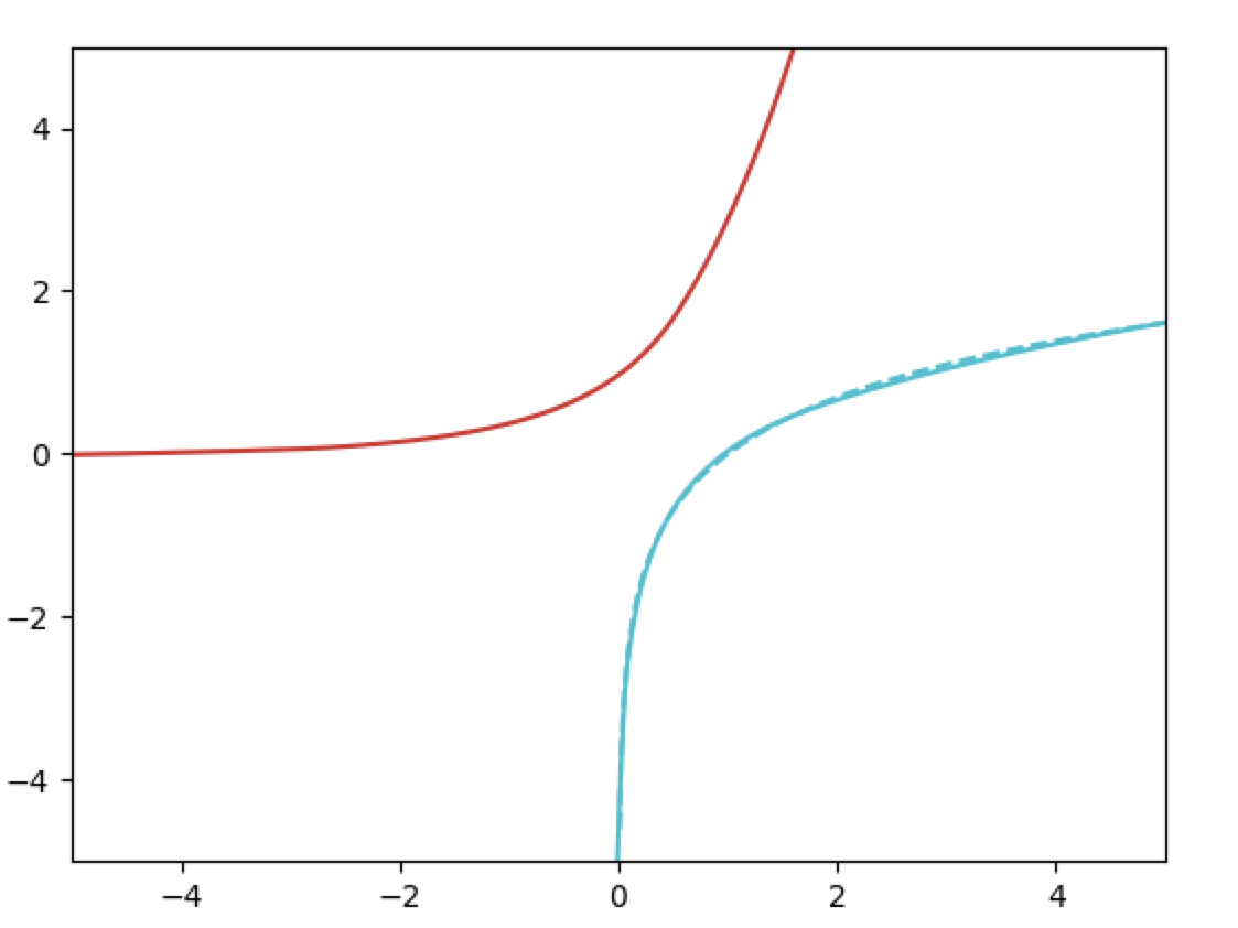
The following plot shows a InvertibleNN trained to represent $\log(x)$. The dotted line is the ground truth, the blue line is the learned forward function, and the red line is the inverse function. Note that the inverse is not explicitly trained, but it still converges to $e^x$.

It is extremely straightforward to use GenAgg in existing GNN architectures. Simply set the aggr attribute of your GNN layer to an instance of GenAgg:

edge_index = torch.tensor([[0, 1, 1, 2],
                           [1, 0, 2, 1]], dtype=torch.long) # 2 x num_edges
x = torch.rand(3,2) # num_nodes x feature_dim
data = Data(x=x, edge_index=edge_index)
agg = GenAgg() # init GenAgg
gnn = GraphConv(in_channels=2, out_channels=1, aggr=agg) # init GNN with GenAgg
y = gnn(x=x, edge_index=edge_index) # evaluate
print("x:", x)
print("y:", y.detach())

x: tensor([[0.5977, 0.9049],
          [0.6357, 0.4703],
          [0.2521, 0.6275]])

y: tensor([[0.1559],
          [1.2240],
          [0.1208]])

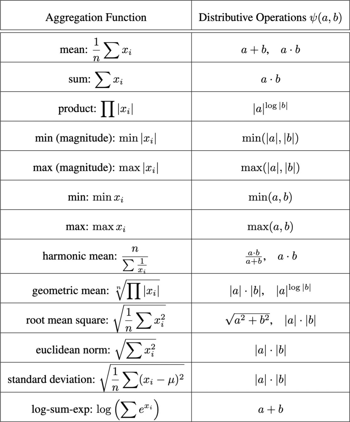
Generalised Distributive Property

Given our generalised parametrisation of aggregation functions, we also define a generalised distributive property—just as the standard distributive property states $\sum c x_i = c\sum x_i$, we define a distributive property for any aggregator. This is particularly useful when developing efficient algorithms. Just as the Fast Fourier Transform and the Viterbi algorithm use the distributive property to optimise time-efficiency, new approaches can use the generalised distributive property to design efficient algorithms that are not limited by linearity.

Generalised Distributive Property. For a binary operator $\psi$ and set aggregation function $\bigodot$, the Generalised Distributive Property is defined:

$$\psi \left(c, \bigodot_{x_i \in \mathcal{X}} x_i \right) = \bigodot_{x_i \in \mathcal{X}} \psi(c, x_i)$$

Theorem. For GenAgg parametrised by $\theta = \langle f, \alpha, \beta \rangle = \langle f, \alpha, 0 \rangle$, the binary operator $\psi$ which will satisfy the Generalised Distributive Property for $\bigoplus_\theta$ is given by: $$\psi(a,b) = f^{-1}(f(a) \cdot f(b))$$ Furthermore, for the special case $\theta = \langle f, \alpha, \beta \rangle = \langle f, 0, 0 \rangle$, an additional solution is: $$\psi(a,b) = f^{-1}(f(a) + f(b))$$

While the proof can be found in our paper, we demonstrate this numerically with GenAgg:

f = InvertibleNN()
agg = GenAgg(f=f)
x = torch.randn(10)
c = torch.randn(1)
yc1 = agg.dist_op(c, agg(x, dim=0))
yc2 = agg(agg.dist_op(c, x), dim=0)
print("c˚agg(xi):", yc1.detach())
print("agg(c˚xi):", yc2.detach())

c˚agg(xi): tensor([6.4132])

agg(c˚xi): tensor([6.4132])